The next project was completed using the Fashion-MNIST dataset and PyTorch to build a neural network. There is a GitHub link to a notebook with a more detailed version of this project provided at the bottom.
PyTorch was something I had not previously explored so I decided this image classification problem would be a good use-case to try it out.
Load the dataset and explore
The first thing I did was use the data loaders to load in the data and normalise it all. This was achieved as follows.
#Set a batch size, this is 0.2% of training data
#Ideally I wanted this higher but I had memory errors
batchSize=10
#Create a transformer to normalize the image
transform = transforms.Compose([transforms.ToTensor(), transforms.Normalize((0.5,), (0.5,))])
#Load the training data
trainset = datasets.FashionMNIST(root='./data', train=True,
download=True, transform=transform)
trainloader = torch.utils.data.DataLoader(trainset, batch_size=batchSize,
shuffle=True, num_workers=2)
#This trainloader doesn't shuffle so it can be used for working out training accuracy
trainloader_ns = torch.utils.data.DataLoader(trainset, batch_size=batchSize,
shuffle=False, num_workers=2)
#Load the test data
testset = datasets.FashionMNIST(root='./data', train=False,
download=True, transform=transform)
testloader = torch.utils.data.DataLoader(testset, batch_size=batchSize,
shuffle=False, num_workers=2)
#Create the class labels
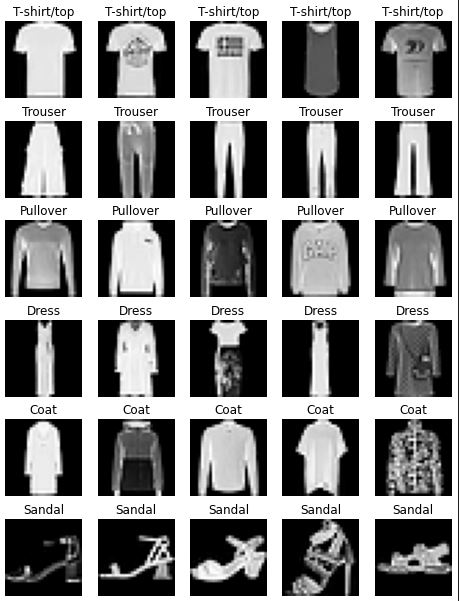
classes = ('T-shirt/top', 'Trouser', 'Pullover', 'Dress', 'Coat', 'Sandal', 'Shirt', 'Sneaker', 'Bag', 'Ankle boot')
I then used matplotlib to print out some examples and observe what they looked like in the grey scale.
#Create figure
fig = plt.figure(figsize=(8,18))
columns = 5
rows = 10

#Set some lists to append to
image_list = []
class_list = []

#Loop thorugh each class
for cl in classes:
    class_count = 0
    #While we haven't found 5 of that class, loop and add images
    while class_count < 5:
        img_xy = np.random.randint(len(trainset))
        if cl == classes[trainset[img_xy][1]]:
            img = trainset[img_xy][0][0,:,:]
            image_list.append(img)
            class_list.append(cl)
            class_count += 1

#Display the images
for i in range(1, columns*rows +1):
    fig.add_subplot(rows, columns, i)
    plt.axis('off')
    plt.title(class_list[i-1])
    plt.imshow(image_list[i-1], cmap='gray')
plt.show()
The two things I decided to try were a logistic regression class and then a Convolutional Neural Network on the data. I will start with the Logistic Regression.
Logistic Regression
Logistic Regression can be modeled as an extremly simple neural network with just one node inside of it. I impletemendted this with the following class using PyTorch. This code defines the network, creates the pass forward method, a train method which calls this forward method and finally a method to call predictions on with a trained version of it’s self.
class LogisticRegression(torch.nn.Module):

    #Create the model with one basic layer, 10 class outputs
    def __init__(self):
        super(LogisticRegression, self).__init__()
        self.linear = torch.nn.Linear(28*28, 10)

    #Create our forward pass learning step
    def forward(self, x):
        #Flatten the image
        x = x.reshape(-1, 784)
        y_pred = torch.sigmoid(self.linear(x))
        return y_pred

    #Train the model with the batch
    def train(self, batch, criterion):
        #Split the batch
        images, labels = batch
        #Generate the predictions
        y_pred = self(images)
        #Calcualte our loss
        loss = criterion(y_pred, labels)
        return loss

    #Get the predictions of a dataset using the model
    def get_all_preds(self, data):
        with torch.no_grad():
            total_preds = []
            for batch in data:
                images, labels = batch
                y_pred = self(images)
                _, predicted = torch.max(y_pred, 1)
                predicted = predicted.numpy()
                total_preds.append(predicted)
        return np.concatenate(total_preds).ravel()
I needed a few more things before I could implement this class and these were a way to fit the model, calculate accuracy and generate a confusion matrix.
#Train the model and return it for use
def fit(model, criterion, epochs, optimizer, x_data):
    running_loss = 0.0
    time1 = datetime.datetime.now()
    for epoch in range(epochs):
        for batch in x_data:
            optimizer.zero_grad()
            #Train the model
            loss = model.train(batch, criterion)
            #Backprop
            loss.backward()
            optimizer.step()
            # print statistics
            running_loss += loss.item()
        print(running_loss)
        running_loss = 0.0
    print('Finished Training!')

    #Calculate time taken
    time2 = datetime.datetime.now()
    time_taken = time2-time1
    time_list.append(time_taken)
    print("M3 - Time taken to train is:", (time_taken))

    #Calcualte the number of model params
    model_parameters = filter(lambda p: p.requires_grad, model.parameters())
    params_count = sum([np.prod(p.size()) for p in model_parameters])
    print("M4 - Total trainable params is:", params_count)
    params_count_list.append(params_count)
    return model

#Given two sets of labels as numpy arrays, give accuracy score
def accuracy(predictions, labels):
    total = 0
    correct = 0

    for i in range(predictions.shape[0]):
        if predictions[i] == labels[i]:
            correct += 1
        total += 1
    acc_str = "The accuracy is: " +  str((correct/total)*100) + "%"
    return acc_str

#Given two sets of labels as numpy arrays, create and show a CM
def conf_matrix(ground_truth, predictions):
    cm = confusion_matrix(ground_truth, predictions)

    df_cm = pd.DataFrame(cm, classes, classes)
    plt.figure(figsize=(10,7))
    sn.set(font_scale=1.4) # for label size
    sn.heatmap(df_cm, annot=True, annot_kws={"size": 16}, fmt='g') # font size

    plt.show()
Now all of this was in place I simply created an object of the class, chose Stochastic Gradient Descent to optimise with, set the loss function as Cross Entropy, trained the model and returned the results.
#Create the class
LR = LogisticRegression()
#Set my optimizer as Stocastic Gradient Descent and set hyper params
optimizerLR = optim.SGD(LR.parameters(), lr=0.001, momentum=0.9)
#Set the criterion
criterionLR = nn.CrossEntropyLoss()

#Train the model
epochs = 5
train_model = fit(LR, criterionLR, epochs, optimizerLR,trainloader)

#Get the predictions needed for results
train_output = train_model.get_all_preds(trainloader_ns)
test_output = train_model.get_all_preds(testloader)

#Get ground truth labels
x_true = (trainset.targets).numpy()
y_true = (testset.targets).numpy()

#Print asked for results
test_acc = accuracy(test_output,y_true)
print("M2", test_acc)

#print Confusion Matrix
conf_matrix(y_true, test_output)
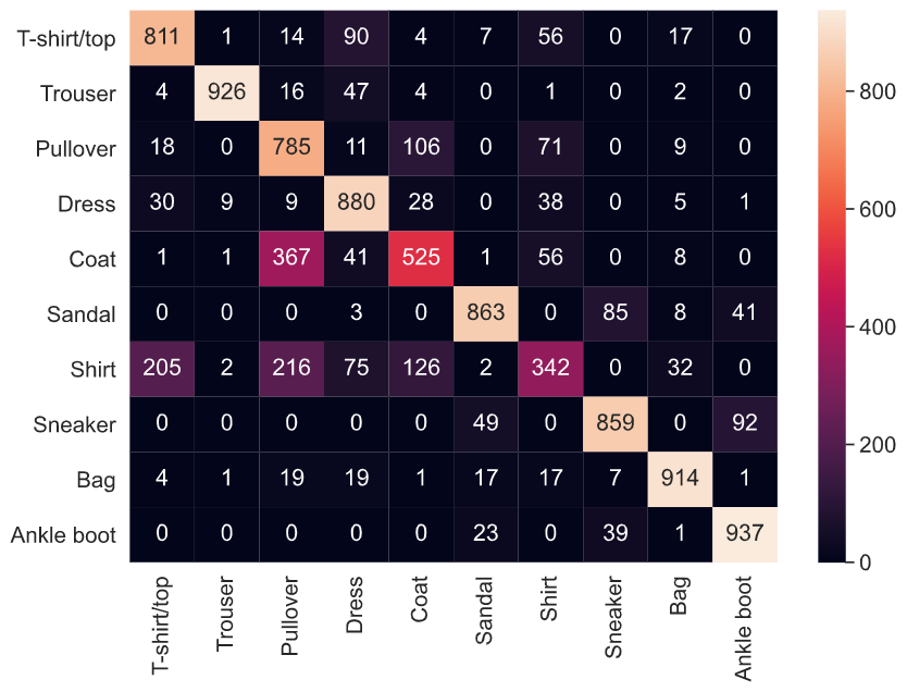
This gave me an accuracy of around 80% in 40 seconds of training time and just 5 epochs, below I will show the confusion matrix generated with seaborn.
These results were a good start but I decided to go one step further and use a CNN.
Convolutional Neural Network
I started again by generating the class that I would need.
#Create a CNN class to use for part A
class CNN(nn.Module):
    def __init__(self):
        super(CNN, self).__init__()
        self.conv1 = nn.Conv2d(1, 8, 5) #3: #input channels; 6: #output channels; 5: kernel size
        self.pool = nn.MaxPool2d(2, 2)
        self.conv2 = nn.Conv2d(8, 16, 5)
        self.fc1 = nn.Linear(16 * 4 * 4, 200)
        self.fc2 = nn.Linear(200, 10)

    def forward(self, x):
        x = self.pool(F.tanh(self.conv1(x)))
        x = self.pool(F.tanh(self.conv2(x)))
        x = x.view(-1, 16 * 4 * 4)
        x = F.tanh(self.fc1(x))
        x = self.fc2(x)
        return x

    #Train the model with the batch
    def train(self, batch, criterion):
        #Split the batch
        images, labels = batch
        #Generate the predictions
        y_pred = self(images)
        #Calcualte our loss
        loss = criterion(y_pred, labels)
        return loss

    #Get the predictions of a dataset using the model
    def get_all_preds(self, data):
        with torch.no_grad():
            total_preds = []
            for batch in data:
                images, labels = batch
                y_pred = self(images)
                _, predicted = torch.max(y_pred, 1)
                predicted = predicted.numpy()
                total_preds.append(predicted)
        return np.concatenate(total_preds).ravel()
I already had the utility functions from above so I again set my optimiser and the loss and trained the model in the exact same way.
myCNN = CNN()

#Set my optimizer as Stocastic Gradient Descent and set hyper params
optimizerCNN = optim.SGD(myCNN.parameters(), lr=0.001, momentum=0.9)
#Set the criterion
criterionCNN = nn.CrossEntropyLoss()

#Train the model
epochs = 5
train_model = fit(myCNN, criterionCNN, epochs, optimizerCNN, trainloader)

#Get the predictions needed for results
train_output = train_model.get_all_preds(trainloader_ns)
test_output = train_model.get_all_preds(testloader)

#Get ground truth labels
x_true = (trainset.targets).numpy()
y_true = (testset.targets).numpy()

#Print asked for results
test_acc = accuracy(test_output,y_true)
print("M2", test_acc)

#print Confusion Matrix
conf_matrix(y_true, test_output)
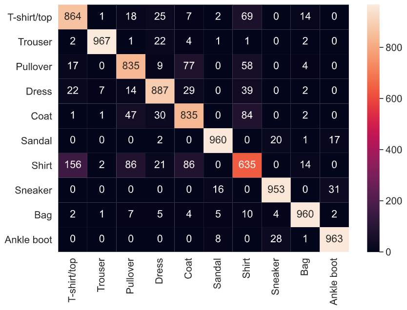
This created a much higher score of 89% in just 2 minutes of training and produced the following confusion matrix.
Conclusion
PyTorch is great? Tensors are totally fantastic and the way it supports itself by calculating back-prop extremely quickly allows CNN’s to be built and work extremely quickly without much training at all. I learnt effective ways of using this package to optimise and solve a quick supervised learning project with it.
