One thing I had not attempted yet in Machine Learning was unsupervised learning. I decided to use Fashion-MNIST again (usuing only 2 classes which were pullovers and jackets) and try some basic techniques on this data set with scikit-learn and PyTorch. There is a GitHub at the bottom linking to a notebook that is more detailed and interactive.
PCA
PCA can be used to create feature reduction in a dataset to stop computational explosion. I started by finding the top 20 components and then visually displaying these with the variance they captured about the data
#Import PCA
from sklearn.decomposition import PCA

#Load the training data for my first class
trainset_class_1 = datasets.FashionMNIST(root='./data', train=True,
                                        download=True, transform=transform)

#Load the training data for my second class
trainset_class_2 = datasets.FashionMNIST(root='./data', train=True,
                                        download=True, transform=transform)

#Select the class that is a pullover
idx = trainset.targets==2

trainset_class_1.targets = trainset.targets[idx]
trainset_class_1.data = trainset.data[idx]

#Select the class that is a coat
idx = trainset.targets==4

trainset_class_2.targets = trainset.targets[idx]
trainset_class_2.data = trainset.data[idx]

#Flatten the class data
class1_data = torch.flatten(trainset_class_1.data, start_dim=1)
class2_data = torch.flatten(trainset_class_2.data, start_dim=1)

#Make a tensor with all the data
all_data = torch.cat([class1_data,class2_data])

#Run PCA and get the 20 components
pca = PCA(n_components=20)
out = pca.fit(all_data).transform(all_data)
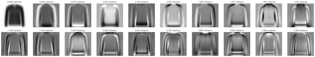
As you can see these don’t really show a lot due to the similar nature of these classes, however it was interesting to see the top Principal Components. Using these I took the top two components going forward to complete my dimensionality reduction.
K-Means
Taking these two top components I scattered the data on a plot to visualise how they looked.

The above shows data that is very close and will be near impossible to cluster in a two dimensional space due to over lapping. Never the less I proceeded on wards to show how the algorithm works and how it can be used.
from sklearn.cluster import KMeans

#Do K-Means
kmeans = KMeans(init='k-means++', n_clusters=2, n_init=10)
kmeans.fit(X_r)

y_kmeans = kmeans.predict(X_r)
centers = kmeans.cluster_centers_

As we can see the algorithm has performed poorly but it was a good learning experience for how to implement it. I learnt more about scikit-learn and finding things that are broken is always a chance to learn for next time.
Auto-Encoder with PyTorch
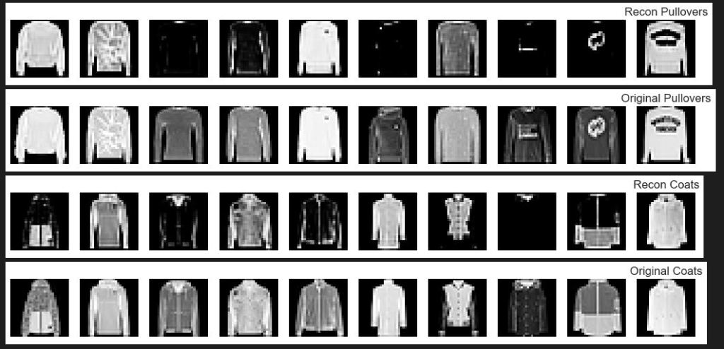
Finally I decided to try an auto-encoder with PyTorch out. Below is the class implementation and then finally is the re-generated images that were created when compared to the originals. This performed much better than PCA reconstuction.
#Declare an Autoencoder class
class Autoencoder(nn.Module):
    def __init__(self):
        super(Autoencoder, self).__init__()
        self.encoder = nn.Sequential(
            nn.Conv2d(1, 8, 3),
            nn.Tanh(),
            nn.Conv2d(8, 16, 3),
            nn.Tanh(),
            nn.Conv2d(16, 32, 3),
            nn.Tanh(),
            nn.Conv2d(32, 64, 3),
        )
        self.decoder = nn.Sequential(
            nn.ConvTranspose2d(64, 32, 3),
            nn.Tanh(),
            nn.ConvTranspose2d(32, 16, 3),
            nn.Tanh(),
            nn.ConvTranspose2d(16, 8, 3),
            nn.Tanh(),
            nn.ConvTranspose2d(8, 1, 3),
            nn.Sigmoid()  #to range [0, 1]
        )

    def forward(self, x):
        x = self.encoder(x)
        x = self.decoder(x)
        return x
Conclusion
I have much to advance with this type of learning still but it was good to make a start. A lot of the issues surrounding PCA were due to the data and a more complex dimensionality may have helped the issue with creating clusters. A more detailed look can be found out below.
